Usage
This section aims to illustrate the benefits of oflibnumpy with examples. In all sample code, it is assumed that the
library was imported using the command import oflibnumpy as of, and therefore the flow class can be accessed using
of.Flow and the functions using of.<function>. All the main examples use class methods instead of the
alternative array-based functions. These work much the same way, but are more limited in their capabilities and
therefore do not illustrate the full scope of oflibnumpy. For some examples, see the section “Array-Based Functions”.
There is an equivalent flow library called Oflibpytorch, mostly based on PyTorch tensors. Its code is available on Github, and the documentation is accessible on ReadTheDocs. This can be advantageous for fast operations, potentially on GPU, when the flow fields are output as a CUDA tensor e.g. by a PyTorch-based deep learning algorithm.
The Flow Object
The custom flow object introduced here has three attributes: vectors vecs, reference
ref (see the section “The Flow Reference”), and mask mask
(see the section “The Flow Mask”). It can be initialised using just a numpy array containing the flow vectors,
or using one of three special constructors:
zero()requires a desired shape \((H, W)\), and optionally the flow reference or a mask. As the name indicates, the vectors are zero everywhere.from_matrix()requires a \(3 \times 3\) transformation matrix, a desired shape \((H, W)\), and optionally the flow reference or a mask. The flow vectors at each location in \(H \times W\) are calculated to correspond to the given matrix.from_transforms()requires a list of transforms, a desired shape \((H, W)\), and optionally the flow reference or a mask. The given transforms are converted into a transformation matrix, from which a flow field is constructed as infrom_matrix().from_kitti()loads the flow field (and optionally the valid pixels) fromuint16pngimage files, as provided in the KITTI optical flow dataset.from_sintel()loads the flow field (and optionally the valid pixels) fromflofiles, as provided in the Sintel optical flow dataset.
Flow objects can be copied with copy(), resized with resize(), padded
with pad(), and sliced using square brackets [] analogous to numpy slicing, which calls
__get_item__() internally. They can also be added with +, subtracted with -, multiplied
with *, divided with /, exponentiated with **, and negated by prepending -. However, note that using
the standard operator + is not the same as sequentially combining flow fields, and the same goes for a
subtraction or a negation with -. To do this correctly, use combine_with() (see the section
“Combining Flows”).
Visualisation
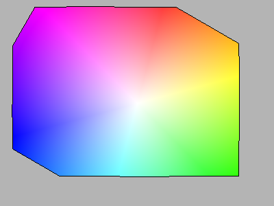
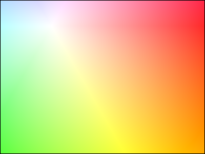
The method visualise() returns a common visualisation mode for flow fields: the hue encodes the
flow vector direction, while the saturation encodes the magnitude. Unless a different value is passed, the maximum
saturation will correspond to the maximum magnitude present in the flow field. show() is a
convenience function that will display this visualisation in an OpenCV window using cv2.imshow(), useful e.g. for
debugging purposes. Note that the flow vectors, i.e. the attribute vecs, are encoded in
“OpenCV convention”: vecs[..., 0] is the horizontal component of the flow, vecs[..., 1] the vertical.
# Get an image of the flow visualisation definition in BGR colour space
flow_def = of.visualise_definition('bgr')

# Define a flow as a clockwise rotation and visualise it in BGR colour space
shape = (601, 601)
flow = of.Flow.from_transforms([['rotation', 601, 601, -30]], shape)
flow_img = flow.visualise('bgr')
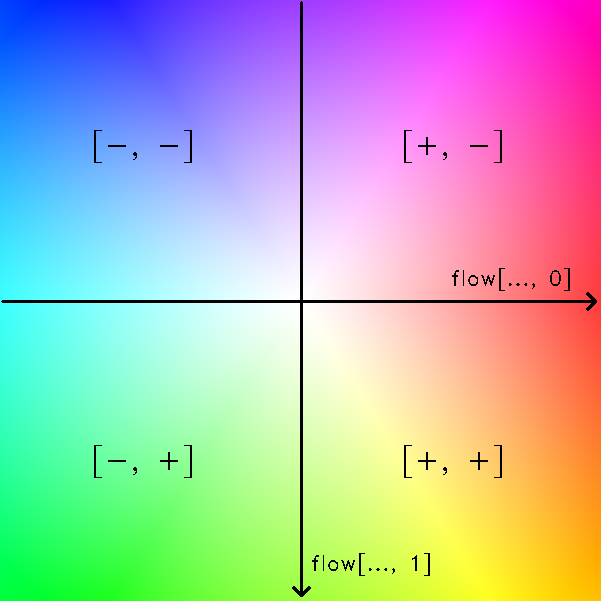

Above: Left: The definition of the flow visualisation, as output by visualise_definition().
Right: the visualisation of a clockwise rotation around the lower right corner.
The visualise() method also offers two parameters, show_mask and show_mask_borders. This
will display the boolean mask mask attribute of the flow object in the visualisation, by
reducing the image intensity where the mask is False, and drawing a black border around all valid (True)
areas, respectively. For an explanation of the usefulness of this mask, see the section “The Flow Mask”.
# Define a flow that is invalid in the upper left corner, and visualise it in BGR colour space
shape = (601, 601)
mask = np.ones((601, 601), 'bool')
mask[:301, :301] = False
flow = of.Flow.from_transforms([['rotation', 601, 601, -30]], shape, mask=mask)
flow_img = flow.visualise('bgr', show_mask=True, show_mask_borders=True)
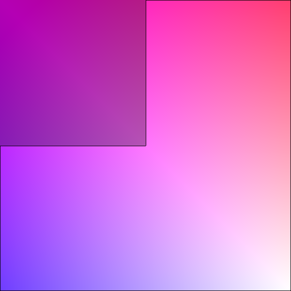
Above: The same clockwise rotation as before, but with a mask that defines the upper left quarter of the flow field
as “invalid”. When show_mask = True, this area has a reduced intensity. show_mask_borders = True adds a black
border around the valid area, i.e. the area where the mask attribute of the flow is True.
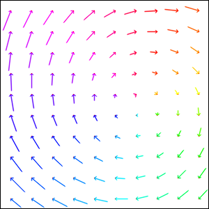
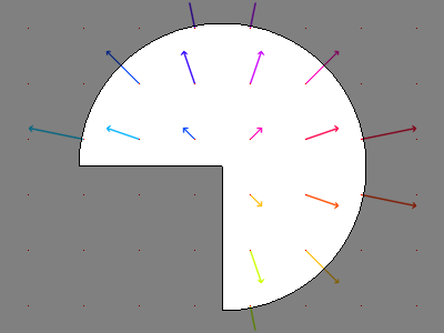
A second, more intuitive visualisation mode is offered in the visualise_arrows() method. Here,
the flow is drawn out as arrows with either their start or end points on a regular grid (see the documentation for the
reference ref flow attribute). The colour of the arrows is calculated the same way as in
visualise() by default, but can be set to a different colour if needed. As with
visualise(), the show_mask and show_mask_borders parameters will visualise the flow mask
mask attribute. And as before, the show_arrows() method is a
convenience function that will display this visualisation in an OpenCV window using cv2.imshow().
# Define a flow as a clockwise rotation and visualise it in BGR colour space as arrows
shape = (601, 601)
flow = of.Flow.from_transforms([['rotation', 601, 601, -30]], shape)
flow_img = flow.visualise_arrows(80)

# Define the same flow, but invalid in the upper left corner, and visualise in BGR colour space as arrows
mask = np.ones((601, 601), 'bool')
mask[:301, :301] = False
flow = of.Flow.from_transforms([['rotation', 601, 601, -30]], shape, mask=mask)
flow_img_masked = flow.visualise_arrows(80, show_mask=True, show_mask_borders=True)
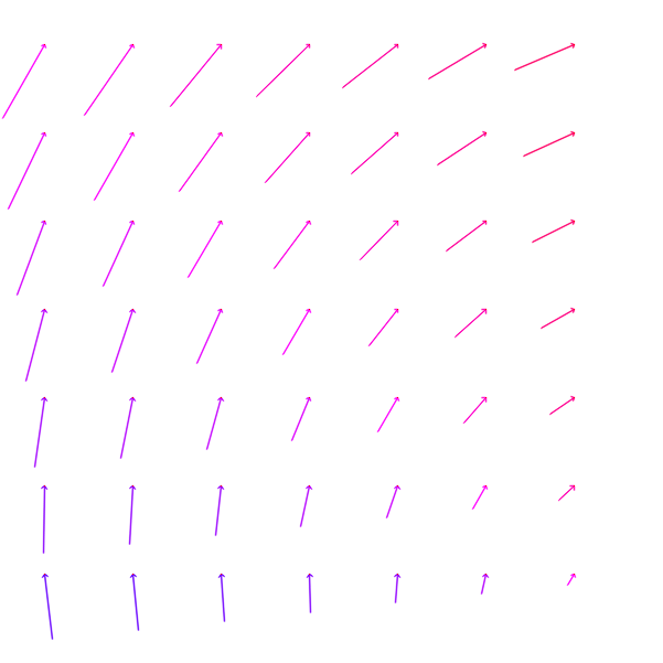
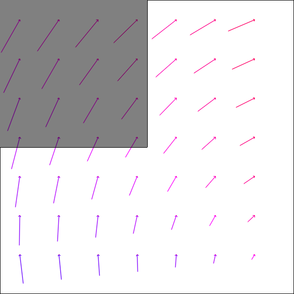
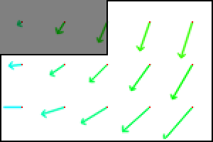
Above: Left: The same flow field as before, a clockwise rotation around the lower right corner, visualised as
arrows. Right: The flow field with the upper left corner defined as “invalid”: this area is visualised with a lower
intensity, and the border of the valid area, where the flow mask attribute mask is True,
is drawn in black
The Flow Reference
The ref attribute determines whether the regular grid of shape H-W associated with the flow
vectors should be understood as the source of the vectors, or the target. So given img1 in the “source”
domain, img2 in the “target” domain, and an associated flow field between the two, there are two possible
definitions or frames of reference for flow vectors:
“Source” reference: The flow vectors originate from a regular grid corresponding to pixels in the area \(H \times W\) in img1, the source domain. They therefore encode the motion that moves image values from this regular grid in img1 to any location in img2, the target domain.
“Target” reference: The flow vectors point to a regular grid corresponding to pixels in the area \(H \times W\) in img2, the target domain. They therefore encode the motion that moves image values from any location in img1, the source domain, to this regular grid in img2.
The flow reference t is the default, and it is significantly faster to warp an image with a flow in that
reference. The reason is that reference t requires interpolating unstructured points from a regular
grid (also known as “backward” or “reverse” warping), while reference s requires interpolating a regular grid
from unstructured points (“forward” warping). The former uses the fast OpenCV remap() function, the latter is
much more operationally complex and relies on the SciPy griddata() function. On the other hand, the
track() method for tracking points (see the section “Tracking Points”) is significantly
faster with a flow in s reference, again due to not requiring a call to SciPy’s griddata() function.
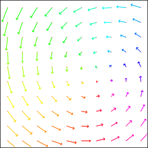
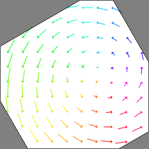
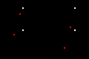
As the images below show, the same rotation will lead to slightly different flow vectors depending on which reference
is chosen. This illustrates that the reference attribute ref cannot simply be set to a
different value if it needs to be changed. For this purpose, the method switch_ref() should be
used. However, this is slow, as it also calls scipy.interpolate.griddata().
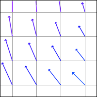
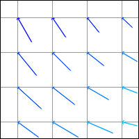
Above: The same rotation with vectors of reference s (left) and t (right). Note that on the left, the
source of the arrows lies on the regular grid drawn in grey, while on the right, the tip of the arrows lies on the
same regular grid.
If the problem is that a specific algorithm that calculates the flow from a pair of images get_flow() is set up
to return a flow field in one reference, but the flow field in the other reference is required, there is a simpler
solution than using the method switch_ref(). Instead of calling
flow_one_ref = get_flow(img1, img2), simply call the algorithm with the images in the reversed order, and multiply
the resulting flow vectors by -1: flow_other_ref = -1 * get_flow(img2, img1). If the flow is needed in both
references, it can even be faster to call get_flow() twice in the way explained above, rather than once and then
using the method switch_ref() once. However, this of course depends on the size of the flow
field, and the operational complexity of the algorithm used to calculate it.
From the previous observations, it also follows that inverting a flow is not a matter of simply inverting the flow
vectors. In flows with reference t, this would mean the target location remains the same while the source switches
to the opposite side, while in flows with reference s, this would mean the source location remains the same while
the target switches to the opposite side. Neither is correct: in actual fact, inverting the flow switches the source and
the target around. This means inverting the flow vectors and changing the reference:
\(F(vecs, t)^{-1} = F(-vecs, s)\) and \(F(vecs, s)^{-1} = F(-vecs, t)\). If the flow is needed with the
original reference, switch_ref() would have to be called. The method
invert() does all this internally, and returns the mathematically correct inverse flow in
whichever reference needed.
# Define a flow
flow = of.Flow.from_transforms([['rotation', 200, 150, -30]], (300, 300), 't')

# Get the flow inverse: in the wrong way, and correctly in either reference
flow_invalid_inverse = -flow
flow_valid_inverse_t = flow.invert('t')
flow_valid_inverse_s = flow.invert('s')
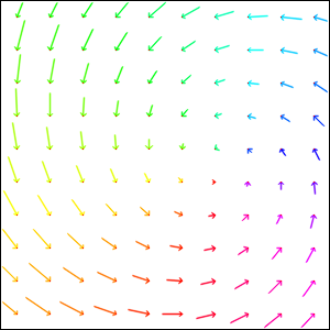
Above: Top: A flow field corresponding to a clockwise rotation in reference t, and the incorrect “inverse”
obtained by simply inverting the flow vectors, also in reference t. Bottom: The correct inverse in reference
s, and the correct inverse in reference t. Note the difference in the flow vectors between the correct and
incorrect inverse - the former describes a pure rotation, while the latter resembles a spiral.
In the images above, the inverse in reference s retains the entire area \(H \times W\) as valid, while the
inverse in reference t has undefined areas. As with the example in the section “The Flow Mask”, this is
not a limitation of the algorithm, but simply a consequence of the operations necessary to invert the flow.
The Flow Mask
The mask attribute is necessary to keep track of which flow vectors in the
vecs attribute are valid. This is useful e.g. when two flow fields are combined (see the
section “Combining Flows”):
# Define two flows, one rotation, one scaling motion
shape = (300, 400)
flow_1 = of.Flow.from_transforms([['rotation', 200, 150, -30]], shape)
flow_2 = of.Flow.from_transforms([['scaling', 100, 50, 0.7]], shape)

# Combine the flow fields
result = flow_1.combine_with(flow_2, mode=3)


Above: Top: Flow 1 (rotation), Flow 2 (scaling). Bottom: Flow combination, plain and masked
The flow visualisations above illustrate how not the entire flow field area \(H \times W\) will actually contain valid or useful flow vectors after a flow combination operation, despite both flow fields used being entirely valid. This is not a limitation of the algorithm, but unavoidable: the scaling operation can be pictured as a “zooming out” motion, which obviously means there will be a “frame” of values that would have had to come from outside of \(H \times W\), and are therefore undefined.
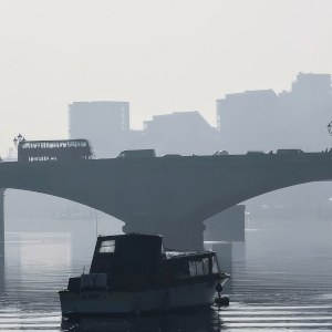
Applying a Flow
The apply() method is used to apply a flow field to an image (or any other numpy array, or indeed
another flow field). Optionally, the valid_area can be returned, which will be True where the warped image
is valid, i.e. contains actual content. For an illustration, see the example below.
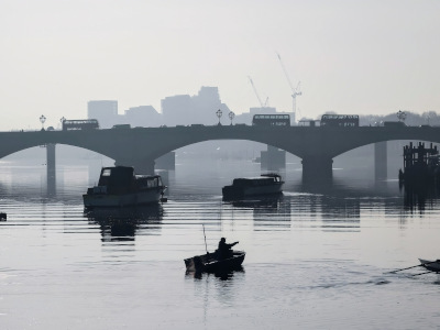
# Load image, and define a flow as a combination of a rotation and scaling motion
img = cv2.imread('thames.jpg')  # 300x400 pixels
transforms = [['rotation', 200, 150, -30], ['scaling', 100, 50, 0.7]]
flow = of.Flow.from_transforms(transforms, img.shape[:2])

# Apply the flow to the image, getting the "valid area"
warped_img, valid_area = flow.apply(img, return_valid_area=True)
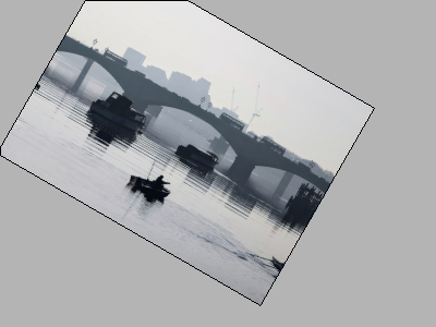
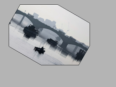
Above: The result of applying a rotation and scaling motion to an image, with the black border showing the outline of
the returned valid_area. As can be seen, the valid area matches the true image content exactly. Left: the flow
field used was the one from the code example above, valid everywhere. Right: the flow field used was the one from the
section “The Flow Mask”, where the valid area is further reduced by the flow field itself having a reduced valid
area.
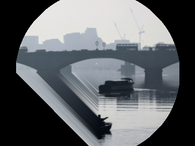
It is also possible to pass an image mask, e.g. a segmentation mask, into the apply() method,
which will be combined with the flow mask to eventually result in the valid_area. This can be useful as in the
example below.
# Make a circular mask
shape = (300, 350)
mask = np.mgrid[-shape[0]//2:shape[0]//2, -shape[1]//2:shape[1]//2]
radius = shape[0] // 2 - 20
mask = np.linalg.norm(mask, axis=0)
mask = mask < radius
# Load image, make two images that simulate a moving telescope
img = cv2.imread('thames.jpg') # 300x400 pixels
img1 = np.copy(img[:, :-50])
img2 = np.copy(img[:, 50:])
img1[~mask] = 0
img2[~mask] = 0
# Make a flow field that could have been obtained from the above images
flow = of.Flow.from_transforms([['translation', -50, 0]], shape, 't', mask)
flow.vecs[~mask] = 0
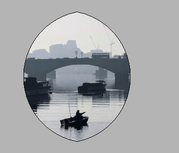
# Apply the flow to the image, setting consider_mask to True and False
warped_img, valid_area = flow.apply(img1, mask, return_valid_area=True)
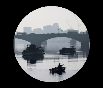
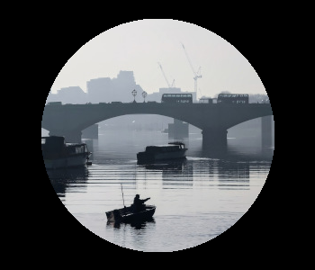
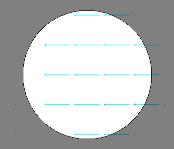
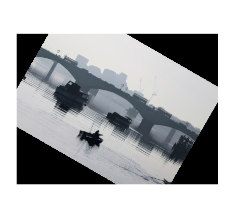
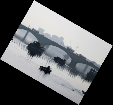
Above: Top: Image 1 and image 2, as they could be seen when looking at the river Thames through a telescope.
Bottom left: The flow field corresponding to the motion from image 1 and image 2, a translation of 50px to the left.
The arrows show clearly that some of the pixels being moved originate outside of the field of view of the telescope,
which means the right-hand-side border of this field of view will be shifted towards the left, reducing the “useful”
image area. This cannot be avoided, as the parts of the image moving into view in image 2 are occluded in image 1.
Bottom right: the result of warping image 1 with the flow field, passing in the telescope field of view segmentation
from image 1 as a mask. The returned valid_area is shown as an overlay, and perfectly matches the location of the true
image content. So while the loss of “true content” area cannot be avoided, it can be tracked by passing the initial
segmentation into the function, and using return_valid_area = True to obtain an updated segmentation.
The examples above use a flow field with reference t. This is the recommended standard for various reasons:
Using
apply()with flow fields of referencesis comparatively slow, as it needs to call SciPy’sgriddata()function.Flow fields of reference
scan contain ambiguities, as vectors from two different locations can point to the same target location. This could happen if there are several independently moving objects in a scene which end up occluding each other. The only way of resolving this is to assign priorities to the flow vectors, which is left to a possible future version ofoflibnumpy.Furthermore, flow fields of reference
sdo not deal well with undefined / invalid flow areas, as the example below shows. One option (the default) considers the flow mask, i.e. ignoring invalid flow vectors, which leads to a smoother result inside the convex hull of the flow target area but risks artefacts appearing. The other option, accessible by settingconsider_mask = False, is to use the invalid vectors anyway, which in this example inserts a lot of black image values in-between the desired image values which are to be interpolated onto the regular grid of the new image: this gets rid of the large artefact visible in the concave area, but does not allow the flow field to expand the image properly. In a future version ofoflibnumpy, this could be at least partially solved by using the default option, but then calculating which image pixels are not in the concave hull, and setting those to zero. However, determining the convex hull of unstructured point clouds brings its own difficulties.
# Make a circular mask with the lower left corner missing
shape = (300, 400)
mask = np.mgrid[-shape[0]//2:shape[0]//2, -shape[1]//2:shape[1]//2]
radius = shape[0] // 2 - 20
mask = np.linalg.norm(mask, axis=0)
mask = mask < radius
mask[150:, :200] = False

# Load image, make a flow field, mask both
img = cv2.imread('thames.jpg')  # 300x400 pixels
flow = of.Flow.from_transforms([['scaling', 200, 150, 1.3]], shape, 's', mask)
img[~mask] = 0
flow.vecs[~mask] = 0

# Apply the flow to the image, setting consider_mask to True and False
img_true = flow.apply(img, consider_mask=True)
img_false = flow.apply(img, consider_mask=False)

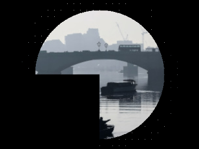
Above: Top: The masked image and the equally masked flow with reference s, corresponding to a scaling motion
from the image centre. Bottom: The result of applying the flow to the image, with / without considering the mask,
i.e. not using / using all flow vector values.
Flow Padding
Given that applying a flow with reference t to an image can lead to undefined areas (as seen in the section
“Applying a Flow”), it can be useful to know how much this image would have to be padded on each side with
respect to the given flow field in order for no undefined areas to show up anymore. A possible application for this
would be the creation of synthetic data for a deep learning optical flow estimation algorithm, with the goal of
obtaining two images and an associated flow field that corresponds to the motion visible between the two images.
The padding can be determined using the get_padding() method, and will be returned as a list of
values [top, bottom, left, right]. If an image padded accordingly is passed to the apply()
method along with the padding values, the image will be warped according to the flow field and automatically cut down
to the size of the flow field, unless the parameter cut is set to False.
# Load an image
full_img = cv2.imread('thames.jpg')  # original resolution 600x800

# Define a flow field
shape = (300, 300)
transforms = [['rotation', 200, 150, -30], ['scaling', 100, 50, 0.7]]
flow = of.Flow.from_transforms(transforms, shape)

# Get the necessary padding
padding = flow.get_padding()

# Select an image patch that is equal in size to the flow resolution plus the padding
padded_patch = full_img[:shape[0] + sum(padding[:2]), :shape[1] + sum(padding[2:])]

# Apply the flow field to the image patch, passing in the padding
warped_padded_patch = flow.apply(padded_patch, padding=padding)

# As a comparison: cut an unpadded patch out of the image and warp it with the same flow
patch = full_img[padding[0]:padding[0] + shape[0], padding[2]:padding[2] + shape[1]]
warped_patch = flow.apply(patch)
Above: Left: The original unpadded image patch. Middle: The unpadded image patch when warped with the same flow field as the one used in the section “Applying a Flow”. Note the similar amount of undefined areas visible in the result. Right: The result of applying the flow to the image patch padded with the necessary amount of padding, and then cut back to size. The padding was just large enough to avoid any undefined areas becoming visible.
For flows with reference s, the above calculation of padding is not possible: after all, the flow vectors express
where pixels in the original image are “pushed” to, rather than where pixels in the warped image are “pulled” from.
Instead, the get_padding() method calculates the padding necessary to ensure no content
is being pushed outside of the image.
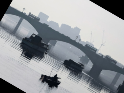
# Load an image, define a flow field
img = cv2.imread('thames.jpg')  # 300x400 pixels
transforms = [['rotation', 200, 150, -30], ['scaling', 100, 50, 0.9]]
flow = of.Flow.from_transforms(transforms, img.shape[:2], 's')  # 300x400 pixels

# Find the padding and pad the image
padding = flow.get_padding()
padded_img = np.pad(img, (tuple(padding[:2]), tuple(padding[2:]), (0, 0)))

# Apply the flow field to the image patch, with and without the padding
warped_img = flow.apply(img)
warped_padded_img = flow.apply(padded_img, padding=padding, cut=False)
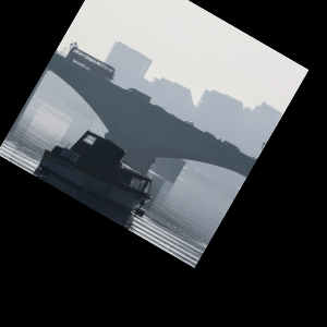
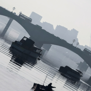
Above: Left: The original image warped with the flow - note the corners that have been moved outside of the image, leading to loss of information. Right: The padded image warped with the flow: the image has been padded the exact amount needed not to lose any image content.
Source and Target Areas
The valid_source() and valid_target() methods both serve to investigate
the flow field. Given an image with the area \(H \times W\) in the source domain and a flow field of the same
shape, applying this flow to the image will give us a warped image in the target domain. Some of the original image
content will no longer be visible after applying the flow: valid_source() returns a boolean
array of shape \((H, W)\) which is False where content “disappears” after warping. The warped image, in turn,
will contain some areas which are undefined, i.e. not filled by any content from the original image:
valid_target() returns a boolean array of shape \((H, W)\) which is False where the
warped image does not contain valid content.
# Define a flow field
shape = (300, 400)
transforms = [['rotation', 200, 150, -30], ['scaling', 100, 50, 1.2]]
flow = of.Flow.from_transforms(transforms, shape)

# Get the valid source and target areas
valid_source = flow.valid_source()
valid_target = flow.valid_target()

# Load an image and warp it with the flow
img = cv2.imread('thames.jpg')  # 300x400 pixels
warped_img = flow.apply(img)

Above: Top: Original image, and the image warped by the flow field. Bottom left: The valid source area - the white area covers the parts of the original image (“source” domain) which are still visible after warping. Bottom right: The valid target area - the white area covers the parts of the warped image (“target” domain) with real image content.
Tracking Points
The track() method is useful to apply the flow field to a number of points rather than an entire
image. In the following example, the int_out parameter is set to True so the new point locations are returned as
(rounded) integers - this is a useful convenience feature if these points should then be plotted on an image. By
default, the method will return accurate float values.
An important point to be aware of is that the track() method is significantly faster for flows
with a “source” reference (ref = 's'), as long as the parameter s_exact_mode is not explicitly set to True.
In this case, no call of SciPy’s slow griddata function is necessary, and instead a fast bilinear interpolation
algorithm is used. This is the recommended usage, at the cost of positional errors in the order of 0.01 pixels.
# Define a background image, sample points, and a sample flow field
background = np.zeros((40, 60, 3), 'uint8')
pts = np.array([[5, 15], [20, 15], [5, 50], [20, 50]])
flow = of.Flow.from_transforms([['rotation', 0, 0, -15]], background.shape[:2], 's')

# Track the points with the flow field, and plot original positions in white, new positions in red
tracked_pts = flow.track(pts, int_out=True)
background[pts[:, 0], pts[:, 1]] = 255
background[tracked_pts[:, 0], tracked_pts[:, 1], 2] = 255
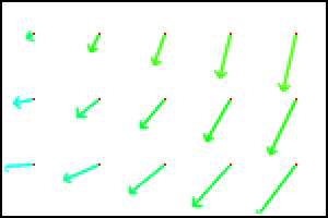
Above: Flow field, and point positions: original points in white, points after applying the flow in red
If the points are rotated more, some will come to lie outside of the image area. In this case, setting the parameter
get_valid_status to True will cause the track() method to return a boolean array which
lists the “status” of each output point. It will be True for any point that was moved by a valid flow vector (see
section “The Flow Mask”) and remains inside the image area.
# Define a background image, sample points, and a sample flow field
background = np.zeros((40, 60, 3), 'uint8')
pts = np.array([[5, 15], [20, 15], [5, 50], [20, 50]])
mask = np.ones((40, 60), 'bool')  # Make a flow mask
mask[:15, :30] = False  # Set the left upper corner of the flow mask to False
flow = of.Flow.from_transforms([['rotation', 0, 0, -25]], background.shape[:2], 's', mask)

# Track the points with the flow field, and plot original positions in white, new positions in red
tracked_pts, valid_status = flow.track(pts, int_out=True, get_valid_status=True)
background[pts[:, 0], pts[:, 1]] = 255
background[tracked_pts[valid_status][:, 0], tracked_pts[valid_status][:, 1], 2] = 255
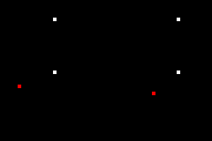
Above: Flow field, and point positions: original points in white, points after applying the flow in red. Note the
upper left and lower right points are missing, as they both have a valid_status of False. For the upper left
point, this is due to the flow vector at that location having been defined as invalid (see the black border in the flow
field visualisation), as the mask used when creating the flow was set to False there. For the lower right point,
this is due to the new location of the point being outside of the image area.
Combining Flows
The combine_with() function was already used in the section “The Flow Mask” with
mode = 3 to sequentially combine two different flow fields. This is a fast operation both for reference s
and t. In the formula \(flow_1 ⊕ flow_2 = flow_3\), where \(⊕\) corresponds to a flow combination
operation, this is equivalent to inputting \(flow_1\) and \(flow_2\), and obtaining \(flow_3\).
However, it is also possible to obtain either \(flow_1\) or \(flow_2\) when the other flows in the equation
are known, by setting mode = 1 or mode = 2, respectively. These operations are comparatively slow due to
calls to SciPy’s griddata(). The calculation will often lead to a flow field with some invalid areas, similar
to the example in the section “The Flow Mask”.
shape = (300, 400)
flow_1 = of.Flow.from_transforms([['rotation', 200, 150, -30]], shape)
flow_2 = of.Flow.from_transforms([['scaling', 100, 50, 1.2]], shape)
flow_3 = of.Flow.from_transforms([['rotation', 200, 150, -30], ['scaling', 100, 50, 1.2]], shape)

flow_1_result = flow_2.combine_with(flow_3, mode=1)
flow_2_result = flow_1.combine_with(flow_3, mode=2)
flow_3_result = flow_1.combine_with(flow_2, mode=3)


Above: Top: Flows 1 through 3. Bottom: Flows 1 through 3, as calculated using
combine_with(), matching the original flow fields. Note that the first flow field
has some invalid areas.
Array-Based Functions
Almost all the class methods discussed above are also available as functions that take numpy arrays representing flow fields as inputs directly. This can appear more straight-forward to use, but they are generally more limited in their scope, and the user has to keep track of potentially changing flow attributes such as the reference frame manually. Valid areas are also not tracked. It is recommended to make use of the custom flow class for anything but the simplest flow operations.
# Define NumPy array flow fields
shape = (100, 100)
flow = of.from_transforms([['rotation', 50, 100, -30]], shape, 's')
flow_2 = of.from_transforms([['scaling', 100, 50, 1.2]], shape, 't')

# Visualise NumPy array flow field as arrows
flow_vis = of.show_flow(flow, wait=2000)

# Combine two NumPy array flow fields
flow_t = of.switch_flow_ref(flow, 's')
flow_3 = of.combine_flows(flow_t, flow_2, 3, 't')

# Visualise NumPy array flow field
flow_3_vis = of.show_flow_arrows(flow_3, 't')